
User Guide — Worked Example
SYNTHETIC DATA — DEMONSTRATION ONLY All effect estimates in this worked example are simulated for demonstration purposes and do not represent results from any published or proprietary analysis. The biological target and outcome panel reflect a real, well-studied drug-target MR design; all numeric values are fictitious.
Overview
This worked example demonstrates the full SEQUOIA-FOREST Plotter workflow for a drug-target MR analysis with two outcome classes: continuous biomarker outcomes (instrument validation panel) and binary disease outcomes (efficacy and safety panel). Because the two panels operate on incompatible x-axis scales; Beta/linear for biomarkers, OR/log for binary diseases, they are built as independent plots and composed in the Faceting Tool.
Dataset
File: IL6R_DEMO_SYNTHETIC_EXTENDED.csv 22 rows · 7 columns
The file contains two logical subsets used to build the two panels. All rows share identical column structure; the distinction between panels is made through the Grouping and Selection filter in the tool, not through separate files.
Columns
| Column | Description |
|---|---|
| Exposure | Drug target (IL6R throughout) |
| Outcome | Disease or biomarker name |
| Analysis | MR method: IVW or Weighted Median |
| nSNP | Number of genetic instruments |
| beta | Effect estimate (log-OR for binary outcomes; SD change for continuous outcomes) |
| SE | Standard error of beta |
| Pvalue | Two-sided p-value |
Data table
Panel A rows — continuous biomarker outcomes (instrument validation)
| Outcome | Analysis | nSNP | beta | SE | Pvalue |
|---|---|---|---|---|---|
| CRP | IVW | 26 | −0.423 | 0.038 | 1.00e−9 |
| CRP | Weighted Median | 26 | −0.401 | 0.047 | 1.74e−8 |
| IL-6 | IVW | 26 | 0.318 | 0.051 | 5.36e−7 |
| IL-6 | Weighted Median | 26 | 0.297 | 0.063 | 2.45e−6 |
| Fibrinogen | IVW | 26 | −0.176 | 0.031 | 1.31e−7 |
| Fibrinogen | Weighted Median | 26 | −0.158 | 0.039 | 5.31e−5 |
| sIL-6R | IVW | 26 | 0.441 | 0.044 | 2.00e−12 |
| sIL-6R | Weighted Median | 26 | 0.418 | 0.055 | 2.74e−11 |
Panel B rows — binary disease outcomes (efficacy and safety)
| Outcome | Analysis | nSNP | beta | SE | Pvalue |
|---|---|---|---|---|---|
| Coronary artery disease | IVW | 26 | −0.186 | 0.046 | 0.0001 |
| Coronary artery disease | Weighted Median | 26 | −0.163 | 0.054 | 0.003 |
| Ischemic stroke | IVW | 26 | −0.128 | 0.049 | 0.011 |
| Ischemic stroke | Weighted Median | 26 | −0.094 | 0.059 | 0.098 |
| Atrial fibrillation | IVW | 26 | −0.041 | 0.045 | 0.381 |
| Atrial fibrillation | Weighted Median | 26 | −0.020 | 0.055 | 0.712 |
| Heart failure | IVW | 26 | −0.139 | 0.050 | 0.005 |
| Heart failure | Weighted Median | 26 | −0.117 | 0.060 | 0.048 |
| Rheumatoid arthritis | IVW | 26 | −0.478 | 0.070 | 3.00e−7 |
| Rheumatoid arthritis | Weighted Median | 26 | −0.431 | 0.086 | 8.10e−6 |
| Type 2 diabetes | IVW | 26 | 0.086 | 0.040 | 0.032 |
| Type 2 diabetes | Weighted Median | 26 | 0.068 | 0.048 | 0.179 |
| Venous thromboembolism | IVW | 26 | 0.191 | 0.059 | 0.001 |
| Venous thromboembolism | Weighted Median | 26 | 0.157 | 0.072 | 0.029 |
The Exposure column (IL6R) is constant across all rows and is not shown in the display tables above; it appears in the full CSV.
Step-by-step workflow
The workflow proceeds in three parts. Steps 1–9 build Panel A (biomarker outcomes). Steps 10–14 reconfigure the same session to build Panel B (disease outcomes). Steps 15–19 compose both panels in the Faceting Tool.
Step 1 — Upload the file
In the File Upload section, drag IL6R_DEMO_SYNTHETIC_EXTENDED.csv onto the upload area or click to browse. After upload, all column headers are available in every mapping and sorting dropdown.

[SCREENSHOT — File upload section: file name IL6R_DEMO_SYNTHETIC_EXTENDED.csv visible, upload confirmed.]
Step 2 — Map data columns
Open Map Data Columns. Assign the five fields as follows. This mapping applies to both panels and does not change between them.
| Field in tool | Column | Notes |
|---|---|---|
| Effect Size | beta | Required. Contains log-OR for binary outcomes and SD-change beta for continuous outcomes. |
| Standard Error | SE | Used to derive 95% CI whiskers. |
| P-Value | Pvalue | Required for significance legend configuration. |
| Y-axis | Outcome | Each row's Y-axis label is the outcome name. |
Set the Y-axis to Outcome. The Analysis column (IVW / Weighted Median) drives sub-row ordering within each group via the Sort configuration in Step 5.
Click Generate Forest Plot.

[SCREENSHOT — Map Data Columns panel: beta → Effect Size, SE → Standard Error, Pvalue → P-Value, Outcome → Y-axis]
Step 3 — Configure axis for Panel A
Open Axis Configuration.
X-axis mode: select Beta — Normal Distribution. All biomarker outcomes are continuous; beta represents SD change in the biomarker per 1 SD reduction in CRP via IL6R variants.
X-axis scale: select Linear.
X-axis range: the default range accommodates the beta values in this panel (approximately −0.6 to +0.6). Adjust custom tick count or range bounds if needed for display.
Reference line: click + Add Reference Line. Set the value to 0, width 1px, style dashed, color black.

[SCREENSHOT — Axis Configuration panel: beta mode selected, linear scale, dashed reference line at x =0]
Step 4 — Filter to Panel A rows
Open Grouping and Selection. Set the grouping column to Outcome.
In the selection filter, deselect all binary disease outcomes (Coronary artery disease, Ischemic stroke, Atrial fibrillation, Heart failure, Rheumatoid arthritis, Type 2 diabetes, Venous thromboembolism), retaining only the four biomarker outcomes: CRP, IL-6, Fibrinogen, sIL-6R.
The plot now shows 8 rows — two rows per biomarker, each representing one MR analysis method. To display the method name on each row, set the Y-axis column to Analysis.

[SCREENSHOT — Plot after filtering: four outcome sections visible, CRP, IL-6, Fibrinogen, sIL-6R only, each with IVW row above Weighted Median row.]
Step 5 — Add visible columns
In Visible Columns, confirm the β (95% CI) and P-Value columns are active and OR is inactive.

[SCREENSHOT — Plot with visible columns: β (95% CI), and P-Value displayed to the right of the markers.]
Step 6 — Add plot title
Open Plot Annotations. Set Main Title to:
Panel A — Instrument validation · Genetically proxied IL-6R inhibition · SYNTHETIC DATA
Position: Top. Alignment: Left. Text size: 11 px.
Set X-axis title to:
Effect Size (95% CI)
Set Description to:
Effect of IL6R genetic instruments on downstream biomarkers, scaled per 1 SD reduction in CRP. Synthetic demonstration dataset — all values are fictitious.

[SCREENSHOT — Plot with title, x-axis label and description visible above the grouped, sorted forest plot.]
Step 7 - Add legend
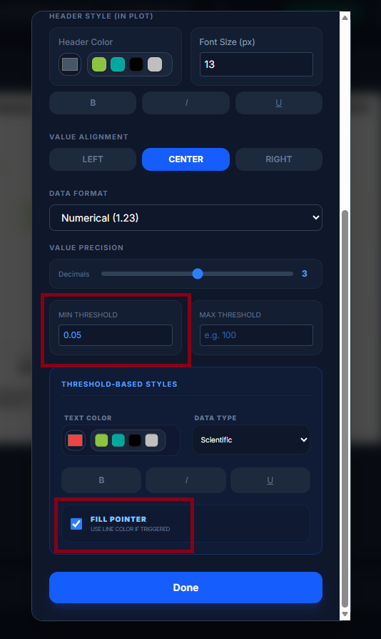
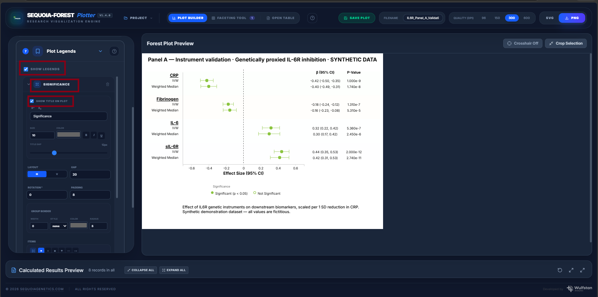
[SCREENSHOT — Plot with significance legend visible at the bottom.]
Step 8 — Adjust plot size
Open Canvas and Display. Adjust the width, height, and margin parameters as required for the figure layout.
Step 9 — Save Panel A
In the toolbar, click Save Plot and enter the filename IL6R_Panel_A_Validation in the dialogue.
Save Plot stores a frozen SVG snapshot of the current plot in the session library, making it available in the Faceting Tool. This is distinct from Save Project, which saves the full configuration state for later reload.

[SCREENSHOT — Save Plot confirmation: plot named IL6R_Panel_A_Validation visible in the left panel of the Faceting Tool sidebar.]
Step 10 — Reconfigure filter for Panel B
Return to Grouping and Selection. Invert the selection: deselect the four biomarker outcomes and reselect all seven binary disease outcomes.
The plot now shows 14 rows — two methods per disease outcome.

[SCREENSHOT — Plot after filter inversion: seven disease outcome sections visible.]
Step 11 — Configure axis for Panel B
Open Axis Configuration.
X-axis mode: select Odds Ratio — Log Distribution. All disease outcomes are binary; the tool exponentiates beta to display OR. Confidence intervals are derived from SE.
X-axis scale: select Log.
The reference line added in Step 5 remains at position 0, which corresponds to OR = 1 on the log scale — the correct null position. The reference line is set to X= 1.

[SCREENSHOT — Axis Configuration panel: Odds Ratio mode selected, Log scale. OR axis visible spanning approximately 0.5 to 1.5.]
Step 12 — Update visible columns
In Visible Columns, enable the OR (95% CI) column while hiding β (95% CI) column (OR mode is active). Confirm OR (95% CI) and P-Value are displayed.

[SCREENSHOT — Plot with OR (95% CI) and P-Value visible.]
Step 13 — Update plot title
Open Plot Annotations. Update Main Title to:
Panel B — Disease risk estimates · Genetically proxied IL-6R inhibition · SYNTHETIC DATA
Update Axis Title to:
OR
Update Description to:
Odds ratios for binary disease outcomes per 1 SD reduction in CRP via IL6R genetic instruments. IVW (primary) and Weighted Median (sensitivity) estimates shown. Synthetic demonstration dataset — all values are fictitious.

[SCREENSHOT — Panel B with updated title and description.]
Step 14 — Save Panel B
Open save plot panel. Enter filename IL6R_Panel_B_Disease. Click Save As Copy (not UPDATE - if UPDATE is selected earlier panel A plot will be replaced by current plot).
Both panels are now saved in the session library and available in the Faceting Tool. Confirm the number represents in faceting tool as 2.

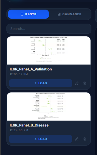
[SCREENSHOT — Both IL6R_Panel_A_Validation and IL6R_Panel_B_Disease visible in the Faceting Tool left sidebar.]
Step 15 — Open the Faceting Tool
Click Faceting Tool in the top navigation bar. The left sidebar shows the Plots library containing both saved plots.

[SCREENSHOT — Faceting Tool open: both saved plots visible in the left sidebar with thumbnails.]
Step 16 — Set canvas dimensions
Click Inspector in the top-right of the toolbar to open the Canvas Settings panel. Set Width to 1400 and Height to 900. Set Background to #ffffff.
These dimensions provide working space for a two-panel vertical composition. The exported file dimensions are computed from the tight bounding box of the placed panels, not from the canvas dimensions set here.

[SCREENSHOT — Canvas Settings panel (open by INSPECTOR): Width 1400, Height 900, Background white.]
Step 17 — Place panels on the canvas
Drag IL6R_Panel_A_Validation from the left sidebar onto the top portion of the canvas.
Drag IL6R_Panel_B_Disease onto the bottom portion of the canvas.
Turn on Snap to Grid in the toolbar before positioning.
Selecting a panel opens the Item Inspector in the right panel. Set the X position identically for both panels so their left edges align. Set Width identically for both panels so their plot areas share the same horizontal span.
Panel A (biomarker, Beta/linear) and Panel B (disease, OR/log) have independent x-axis scales. The two panels are scientifically distinct figures composed into one exhibit, not a shared-axis multi-panel plot.
Resize the canvas using the resize handle at the bottom-right corner of the canvas. Use the zoom controls in the toolbar if necessary.

[SCREENSHOT — Faceting Tool canvas: Panel A positioned above Panel B, left edges aligned, Snap to Grid on.]
Step 18 — Label panels (optional)
Select Panel A in the canvas. In the Item Inspector, enable Show Label, set label text to A, position Top, size 12 px. Repeat for Panel B with label B.

[SCREENSHOT — Item Inspector panel with Show Label enabled.]
Alternatively, panel titles added in Steps 6 and 13 are embedded in the SVG and visible without additional labels.
Step 19 — Export
Select image quality: 600 DPI
Click PNG to export. The exported file dimensions are computed as the tight bounding box of all visible panels plus a fixed 40 px margin — not the canvas Width × Height set in Step 16.
Click SVG to export a vector master file suitable for post-production editing.

[SCREENSHOT — Export controls: DPI selected, PNG and SVG buttons visible. Exported two-panel figure (Figure 19.1).]
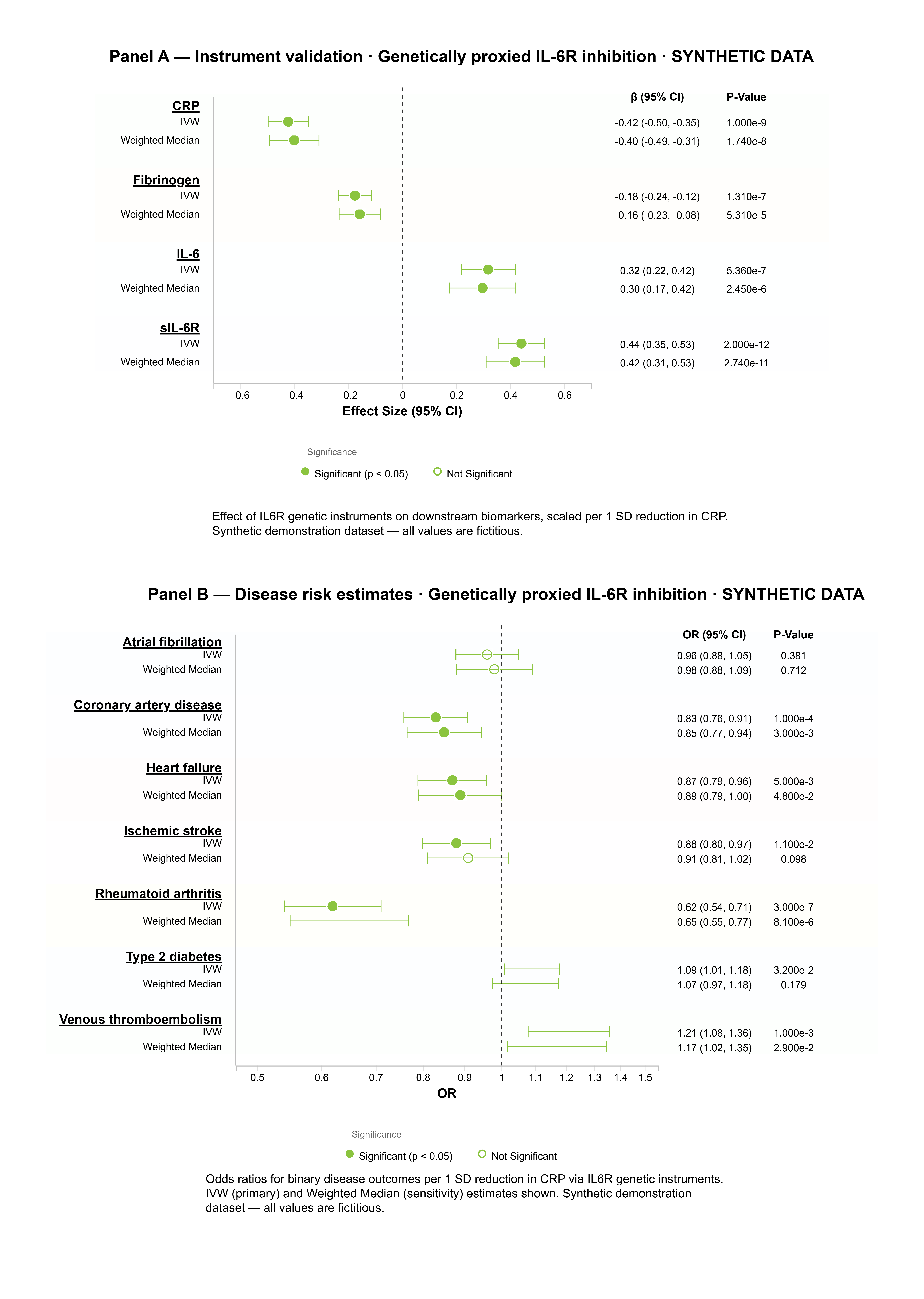
Figure 19.1: Exported two-panel figure
Notes
Save Plot vs Save Project. Save Plot stores a frozen SVG snapshot used by the Faceting Tool. Save Project stores the full configuration state (.seq file) for reloading the interactive session. Both can be used independently. A plot saved with Save Plot does not update automatically if the underlying data or configuration is subsequently changed — re-save to update the Faceting Tool library.
Very small p-values. Rheumatoid arthritis IVW and Weighted Median p-values (3.00e−7, 8.10e−6) may render as 0.000 depending on the decimal precision setting in Visible Columns. This reflects the on-target signal expected when genetically proxying the mechanism of an approved RA drug. If the display truncates to 0.000, adjust column precision or note the scientific notation values in the figure caption.